This post covers the process for the first lab of Studio Northern Grounds (HT20).
For a goal-oriented overview, images corresponding with the specific assignments are listed first. After this introductory overview, the process is presented chronologically.
If you want to jump straight to the process, click one of the following links:
Process entry, 11th of September 2020
Process entry, 13th of September 2020
Process entry, 16th of September 2020
Process entry, 20th of September 2020
Assignments
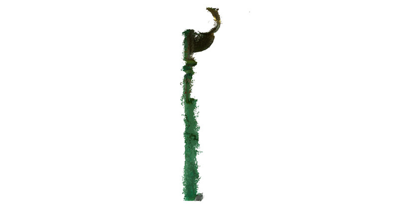
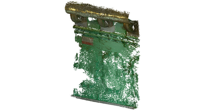
1. 3d scan an interior elevation with intriguing qualities, and create a point cloud of it.
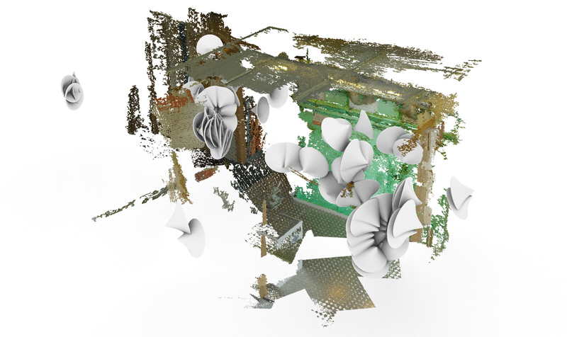
2. Make a diagram showing the camera positions.
3. Make an architectural representation of the point cloud.
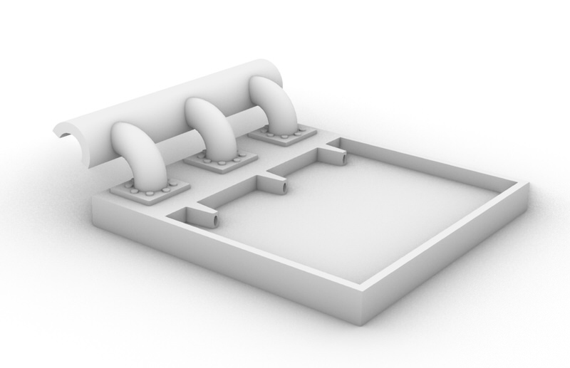
4. With the elevation flipped 90 degrees – rendering it as ground – translate your drawing into a physical model.
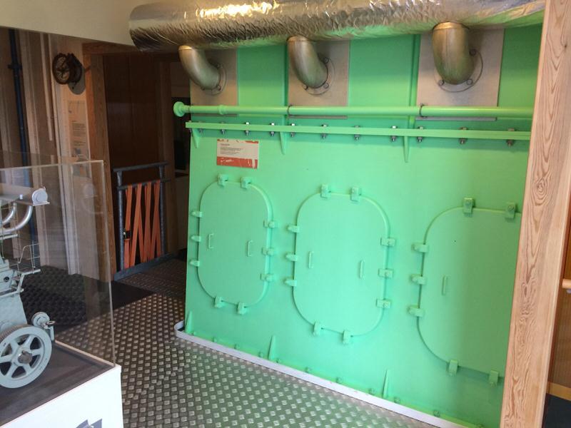
The original intention was to capture a specific interior wall inside the Maritime Museum, the memory of which had intrigued the both of us.
However, upon arrival it was obvious that the wall in mind was far too dark to be captured with our camera – even with maximum ISO (which would have yielded excessive amounts of noise) the environment was too dark. Thus the search for a more brightly lit wall in the museum commenced.
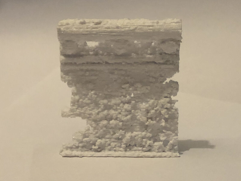
Thus the choice of wall fell upon the most brightly lit interior we could find – which also did have an intriguing aspect of being a replica of a machine room on a modern sea vessel. The quest for a brightly lit room however did distract us from the fact that smooth, untextured surfaces are inappropriate for photogrammetry, since the software will have a hard time identifying distinct details, and even greater difficulty in accurately estimating the location of coplanar points. Although we have dabbled in photogrammetry capture of smaller objects before (the coral, the Stockholm lion, and the sourdough bread on this image are all made with photogrammetry), and ought to have remembered that smooth, untextured surfaces in real-world will produce noisy, spiky surfaces in the reconstructed point cloud, we fell for the machine room wall. It was bland in its materiality, and texture-wise insignificant, but its topology was interesting and intrigued us, in addition to it being relatively brightly lit.
We captured the surface with a DSLR, using the same rigid settings (f/11 for optimum sharpness throughout deep depth of field, 50 mm focal length to reduce distortions to the minimum, etc.) and conventions as we previously had used, working with smaller objects. But with a small object rotated on a Lazy Susan (a small roundabout table) and the camera fixed in its place, it is easy to secure that all angles of the object is captured (and with adequate exposure). For the machine room wall, not so much. The room was very small, and there was little room to move around to capture different angles. Additionally, the rigid limitation of using 50 mm focal depth "for minimum lens distortion" did little to help that in the cramped space, the camera was not allowed to capture a broader view of the wall. This led to the fact that although the 172 photographs surely captured all the wall, only 93 cameras could be aligned in Metashape (presumably due to many photographs not sharing distinguishable details between themselves, being too zoomed in).
With Highest settings for camera alignment, the 93 aligned cameras did only produce 24K tie points, and the sparse point cloud was really sparse.
With High settings for camera alignment, the 93 aligned cameras produced 32K tie points, far more than when aligned with Highest settings. Our hypothesis is that, if we remember correctly, the upsampled images of the Highest settings made it even more difficult for the program to distinguish between signals and noise for the textureless areas, since the upsampling of featureless areas would presumable blend out the captured surface even more, as opposed to theoretically sharpening detailed features. Nonetheless, we went forward with the High settings-alignment.
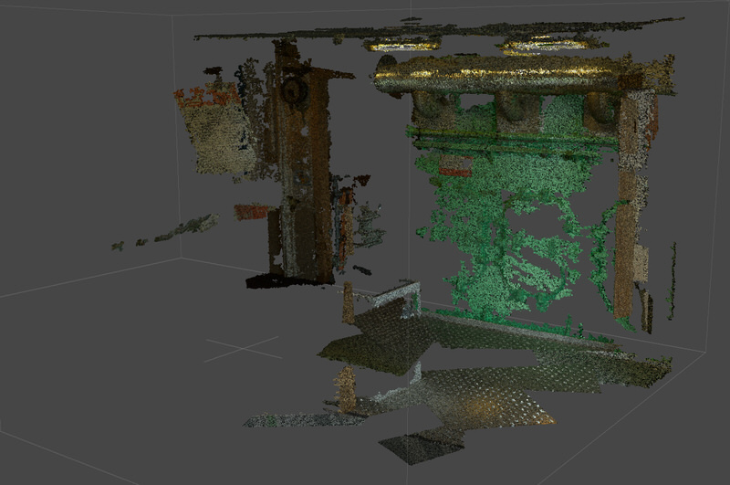
With Ultra High settings for the dense point cloud generation, an impressive 290M points were generated. However, they seemed to be very densely populated in certain areas, and non-existent in others.
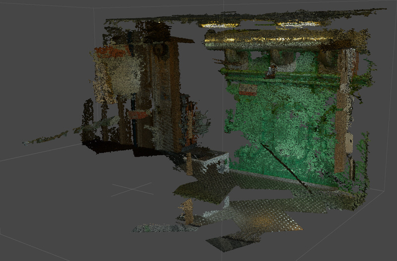
Because of that, we tried to generate another dense point cloud, this time with High settings (as per our experience with the slightly counter-intuitive results of the camera alignment settings). This produced "only" 109M points, about a third of the Ultra High settings output, but the coverage of the surface was significantly better. Some artefacts appeared – like the black rod shooting out from the floor – but generally, the results were better. At least better in terms of the representation of the wall as a whole – there was no doubt that the surface was more noisy than the Ultra High settings output, but it did not have as many gestalt-breaking holes.
Due to the artefacts and the general noisiness found in the High settings output, we presume that the Ultra High settings have a smaller tolerance for deviations and artefacts, but also require better source material to actually realize the potential of the higher settings – otherwise its tightened tolerances are bottlenecked by the lack of (ultra) high quality data.
We imported the dense point cloud to CloudCompare, and while initially quite appalled by the shaggety look of it...
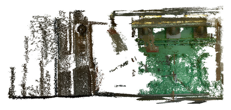
...the feeling was shrugged off when only the primary focus of interest was retained. The result was not of endeavourable quality, but still puts forward the notion we were intrigued by: "we're on a ship!"
In Rhino, we used the Grasshopper definition developed alongside this tutorial to recreate the the correct locations and rotations of the Metashape cameras, and assigned a revolved brep to signify the orientations of cameras. In hindsight, it would have been more accurate to let the revolved brep have a total angle of about 27 degrees – reflecting the 50 mm focal length (in 35 mm film) field of view – instead of the approximately 90 degrees field of view the current cone embodies, but we think that the excessive clustering of the camera locations (due to the cramped space not allowing for much variation) is evident nonetheless. Thus the primary point gets through.
Returning to CloudCompare, we rendered several views of the cropped point cloud for the architectural representation of it. Here, the primary elevation is showed from its front.
Here, it is shown from the left side...
...and here from the bottom.
Here is an isometric view of the cropped point cloud...
...and here is an isometric view of the point cloud, flipped 90 degrees to make it lying as ground. Trying to interpret the elevation in its new identity as ground, we identified an association to flowing water, initially in the form of three distinct waterfalls originating from the large, insulated metal tube, then in the form of whirling water where the noise of the surface increases (where the surface was too smooth to be accurately reconstructe by Metashape).
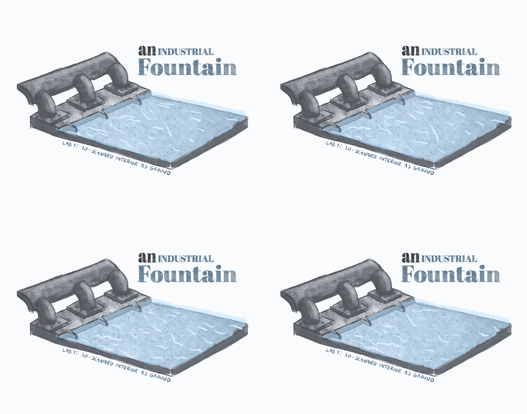
Taking into account favorable and unfavorable conditions for creating a physical model, we decided to follow up on the latter trail (deeming the three large waterfalls less realistic to reproduce in a physical matter), and focused on the noise of the lying surface to be interpreted as water in motion. We produced concept art for a physical model which would function as an underwater fountain of some sort, with water flowing from within the three large pipes into a pool of water, producing whirls in the water representative of noise in the captured point cloud.
The next step will be to take the concept art into the 3D realm, and test if we can produce a physical model with the Anet A8 3D printer we built three years ago, but which has not seen much use since the onset of Manfred. Yesterday night, it was nevertheless brought to a spot where it actually can be used, and we hope to use it as soon as a manifold 3D model has been produced. But for now, we will have to do some reading in the time alloted to us.
The architectural representation produced before the notion of only the elevation being of significance for the lab had been internalised.
From the concept art, we developed a 3D model intended for printing. But initially, the model offered several problematic areas with regards to the production method. Since the 3D printer works in layers, overhangs must be supported, so as not to be printed out in the void.
Instead of relying on automatically generated supports (which could have interfered with the bubble exhaust system), we altered the geometry to fit the production method better. Here no overhangs are unsupported, and the thin support pillars can be removed post-production.
Here the internal exhaust system is showing, making possible the intention to produce noise (in the form of bubbles and whirls).
For 5-6 hours, our 3D printer worked hard while we supervised the development, layer per layer.
Being the first time we 3D printed in more than two years, we were satisfied with the more than adequate results.
And satisfaction turned to joy when we found out that the design worked! It was possible to produce noise in the water by blowing through the exhaust system, creating bubbles and whirls, as well as some extra audio noise. All representing the noisy surface of the captured point cloud.
After tutoring, and being guided in another direction, where the qualities of the point cloud ought to be interpreted not as a gestalt, but for its inherent data, we took some time to improve the representation of the camera locations, while thinking about how to proceed for the physical model. Here it is much more obvious than before that the narrow field of view (27 degrees horizontally, corresponding with our camera setup) really constricts the amount of overlap possible, and that it presumably is co-responsible for the noisy surface, together with its textureless smoothness.
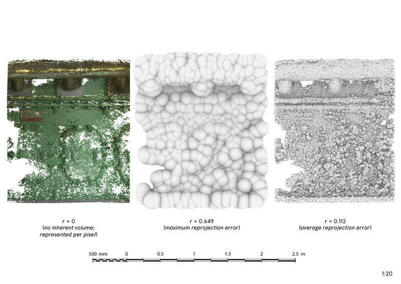
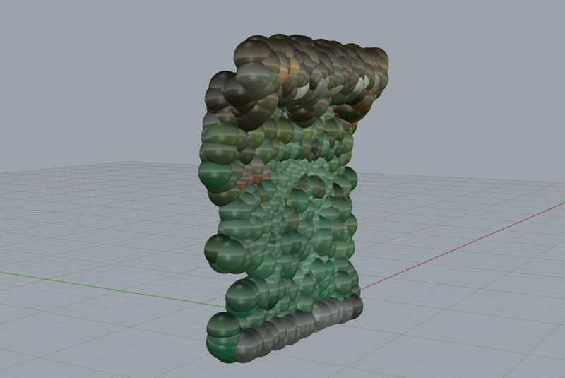
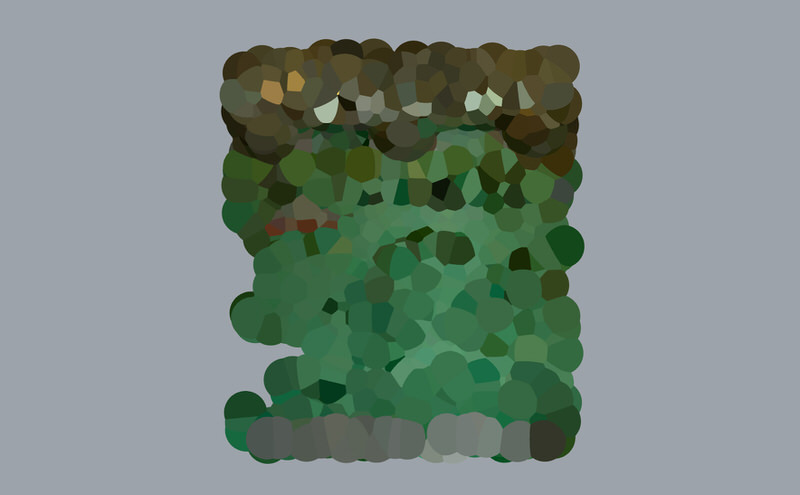
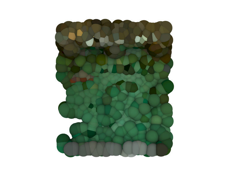
Taking up the noise in itself as the primary variable to proceed with, we decimated the point cloud to a reasonable level for processing times, and spawned a sphere for each remaining point, with its colour defined by the point where it spawned, and with its radius defined by the maximum reprojection error in Metashape. Thus we created a representation of the point cloud where, taking for granted that the maximum reprojection error is correctly reported by Metashape, the point cloud is expanded (per remaining point) to show the large tolerance the maximum reprojection error entails. With a maximum reprojection error as large as this (without the point cloud not yet being in a controlled scale it is non-significant to state, but it was about 0.649 for the point cloud "out of the box"), it is obvious that the representation of the surface allows for much noise.
First we intended to allow for the RGB values to also be included in the new direction the explorations had taken...
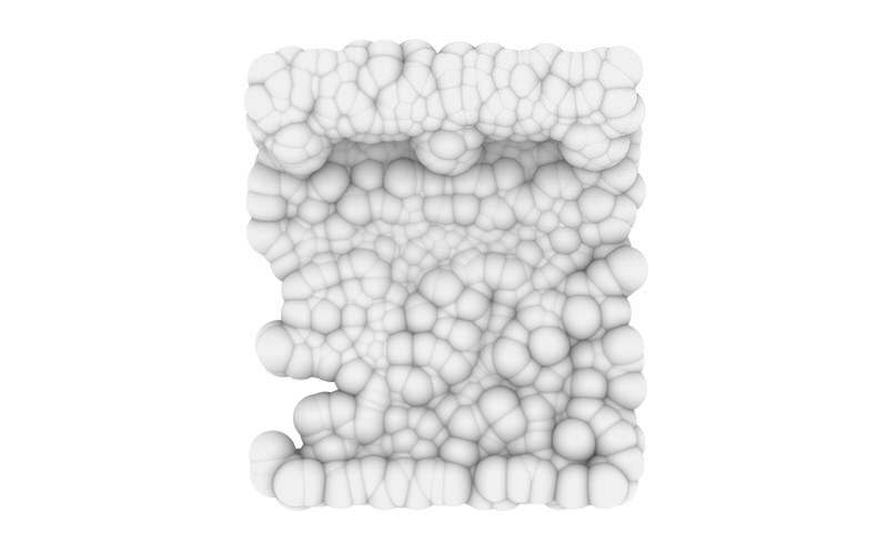
But it was clearly the topology of the noise tolerance landscape that we found most interesting.
So in the end, we chose to focus solely on the topology of the maximum noise tolerance.
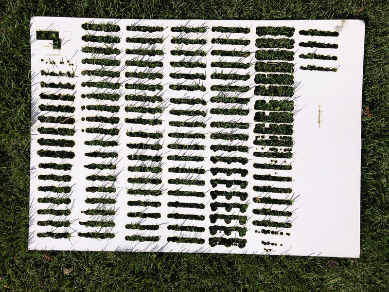
We used section contours of the Rhino model with 1 mm as interval, and 1 mm cardboard as material to use with the laser cutter in the Digital Fabrication Lab at school.
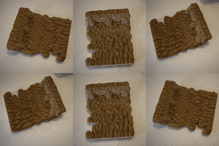
The laser cutter produced some 110 layers, ready to be glued together to reacquire a resemblance to its 3D model form.
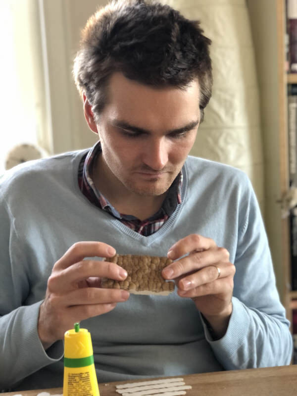
By visiting Grandma with Manfred, we allowed ourselves to focus on the gluing of layers.
And some glimpses of free time inbetween layers.
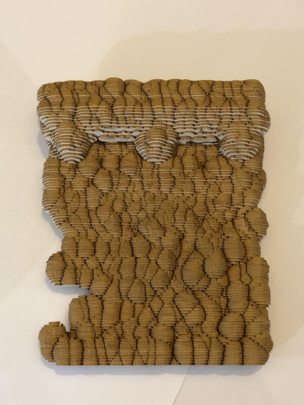
The form of the maximum reprojection error model takes shape.
Although the point cloud has been decimated to a fraction of its original point count (merely 979 points, however representatively distributed in space [due to culling based on distance to other points], in relation to the original 35.5 million points in the cropped point cloud) to allow for the calculations to be feasible in terms of processing time, one can still clearly see the consequence of having the radius of each point set to the maximum reprojection error reported by Metashape. The volume-less point cloud is now represented by a a series of blobs, each representing the sphere, at the center of which its associated point was reconstructed in Metashape, and within the radius of which the point by a statistical certainty the "true" location of the point has to be.
Here the model is presented in its pre-flipped state.
And here it is flipped, considered as ground.
A still of the flipped model.
Next in turn was the physical model representing not the maximum reprojection error, but the reported average reprojection error. Due to the average value being considerable smaller than the maximum value (0.112 vs. 0.649) – which is to be expected – the model required much more points to be retained so as to still produce a representative image of it (48 348 points vs. 979 points).
With both models finished in their digital state, we produced the architectural representation representing the point cloud and the quality we had chosen as our focal point – noise, represented in the form of reprojection error.
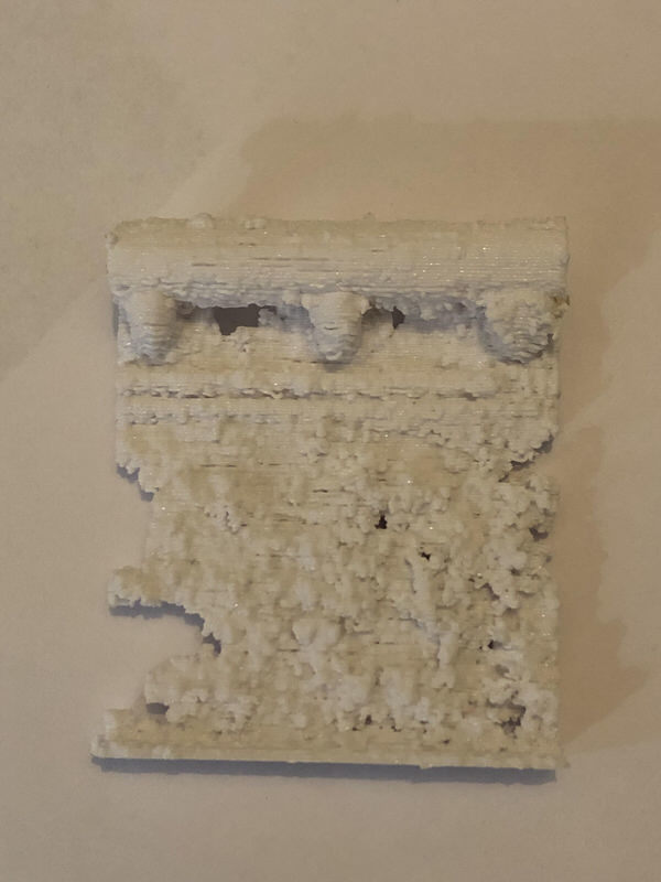
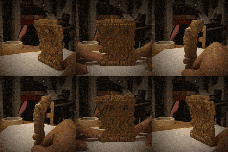
After crashing Rhino and Blender too many times in our quest to produce a manifold mesh of 48 thousand mathematically defined spheres, we decided to simply export the 48 thousand spheres (converted to meshes) directly from Rhino as a Stereolithography (.stl) file, and thankfully it worked – Cura accepted the file contents and processed the mesh accordingly. Due to the fact that a 3D print in the same scale as the laser cut model (1:20) would have taken more than 12 hours (the surveying of which is not compatible with baby life), we chose half the relative scale (1:40), which only took a little more than three hours.
Note to self: generating supports for the 3D print might be crucial for overhang geometry, but if you have the time, model it yourself instead of auto-generating it. If you do auto-generate it, remember that only brute force (and a wire cutter positioned in the right holes) will help you get rid of it.
The 3D printed model in its pre-flipped state.
The flipped model, considered as ground. By a statistical average, most, but not all, of the spheres' associated points are correctly reconstructed within these spheres, but since the radius of the spheres only corresponds with an average value, there are points associated with the spheres which are not correctly reconstructed within the model's physical boundaries. But as a representation of the average value, it holds a more precise representation of the reconstructed point cloud.
If you would like to return to the overview of our Studio Northern Grounds posts, please click here.
